Partial Differential Equations (PDEs) play a foundational role in modeling physical phenomena involving functions of multiple variables—such as heat flow, wave propagation, fluid dynamics, and quantum mechanics. These equations describe how quantities evolve over space and time, often governed by laws of conservation, motion, or energy.
🧩 Types of PDE Problems
Two major classes of problems arise when dealing with PDEs:
• Initial Value Problems (IVPs): Solutions evolve over time from given initial conditions. These are common in time-dependent systems like waves or diffusion.
• Boundary Value Problems (BVPs): Solutions are defined within a spatial domain with specified boundary conditions. These are often encountered in steady-state or spatially constrained scenarios.
🧪 Core Equations and Concepts
Some of the most studied equations in this field include:
• Diffusion Equation: Describes the spread of heat or particles (e.g., heat equation).
• Advection Equation: Describes the transport of material by a velocity field.
• Poisson Equation: A classic elliptic PDE appearing in electrostatics, fluid flow, and gravitational fields.
These core equations provide a foundation for understanding more complex physical systems.
🛠 Numerical Techniques for PDEs
Several numerical techniques are used to discretize and solve PDEs:
• Relaxation Methods: Iteratively approach the solution of elliptic equations like the Poisson equation.
• Fourier-Galerkin Method: A spectral method using orthogonal functions (e.g., sine, cosine) to approximate PDE solutions with high accuracy.
• Stability Analysis: Evaluates the numerical behavior of a method under perturbations or over long time integration.
• Implicit and Explicit Schemes: Methods for time-stepping. Explicit schemes are simple and fast but often require small time steps for stability. Implicit schemes, such as the Crank–Nicolson method, are stable under larger steps but more computationally intensive due to solving matrix systems.
🔗 See more examples here.
🌊 Korteweg–de Vries (KdV) Equation
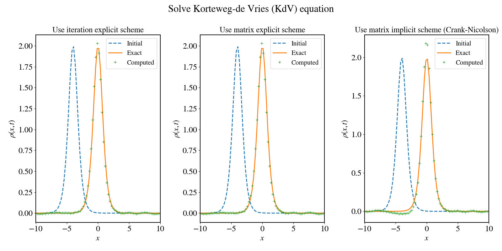
The Korteweg–de Vries (KdV) equation is a nonlinear PDE that models wave motion in shallow water. It combines nonlinear advection with third-order dispersion: $$ \frac{\partial \rho}{\partial t}=-6\rho \frac{\partial \rho}{\partial x} - \frac{\partial ^3 \rho}{\partial x^3}. $$ This equation is renowned for supporting soliton solutions—waves that maintain their shape while propagating at constant speed. In this project, I use Dirichlet boundary conditions, \(\rho(x= L/2)=\rho(x= -L/2)=0\) and test the program with the known solitary wave solution \(\rho(x,t)=2 \mathrm{sech} ^2(x-4t)\).
🔧 Numerical Methods Implemented
To solve the KdV equation numerically, I implemented three approaches:
• Explicit Scheme (Iterative Method): Direct time stepping with finite differences.
• Explicit Scheme (Matrix Method): Matrix formulation for improved computational structure.
• Implicit Scheme (Crank–Nicolson Method): A semi-implicit method with better stability and accuracy.
🔗 See more details here.
Simulation Result
Below is a comparison of wave evolution using different numerical schemes: (From left to right, the time steps \(\tau\) are \(10^{-4}\text{s}\), \(10^{-4}\text{s}\), and \(5 \times 10^{-3}~\text{s}\), respectively.)